토픽 모델링 연습문제
speeches_roh.csv에는 노무현 전 대통령의 연설문 780개가 들어있습니다. speeches_roh.csv를 이용 해 문제를 해결해 보세요.
| library(multilinguer) library(KoNLP) # 명사 추출, extractNoun useNIADic() library(readr) # read_csv 라이브러리 library(dplyr) library(stats) library(stringr) # str_replace_all, str_squish , str_count.... library(textclean) library(tidytext) # 명사 추출 |
1. speeches_roh.csv를 불러온 다음 연설문이 들어있는 content를 문장 기준으로 토큰화하세요.
1-1) 데이터 불러오기
| speeches <- read_csv("C:/speeches_roh.csv") |
1-2) 문장 토큰화 : unnet_tokens 함수
| speeches_comment <- speeches %>% unnest_tokens(input = content, output = sentence, token = "sentences", drop = F ) |
input : 문자열 또는 기호로 분할되는 입력 열
output : 문자열 또는 기호로 만들 출력 열
token : 토큰화를 위한 단위 또는 사용자 지정 토큰화 함수
drop : 원래 입력 열을 삭제해야 하는지 여부입니다. 무시 원래 입력 열과 새 출력 열의 이름이 같은 경우.
2. 문장을 분석에 적합하게 전처리한 다음 명사를 추출하세요.
2-1) 전처리
| speeches_comment <- speeches_comment %>% mutate(sentence = str_replace_all(sentence, "[^가-힣]", " "), sentence = str_squish(sentence)) |
2-2) 명사추출
| nouns_speeches <- speeches_comment %>% unnest_tokens(input = sentence, output = word, token = extractNoun, drop = F) %>% filter(str_count(word) > 1) |
3. 연설문 내 중복 단어를 제거하고 빈도가 100회 이하인 단어를 추출하세요.
3-1) 연설문 내 중복 단어 제거
| nouns_speeches2 <- nouns_speeches %>% group_by(id) %>% distinct(word, .keep_all = T) %>% ungroup() nouns_speeches2 |
ungroup() : 계산을 마쳤을 때 항상그룹 해제()
해줘야 뒷부분에서 단어 빈도수 셀때 올바르게 count 할 수 있다
3-2) 단어 빈도 100회 이하인 단어 추출
| nouns_speeches3 <- nouns_speeches2 %>% add_count(word) %>% filter(n <= 100) %>% select(-n) nouns_speeches3 |
add_count() : 그룹별 카운트로 새열을 추가 # 컬럼 n 생성
filter(n <= 100) : 단어 빈도 100회 이하인 단어 추출
select(-n) : 빈도수 확인하고 n컬럼은 빼고 보여주기
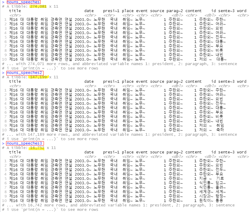
nouns_speeches : 명사 추출한 데이터
nouns_speeches2 : 연설문 내 중복 단어 제거한 데이터
nouns_speeches3 : 단어 빈도 100회 이하인 단어 추출한 데이터
4. 추출한 단어에서 다음의 불용어를 제거하세요.
| stopword <- c("들이", "하다", "하게", "하면", "해서", "이번", "하네", "해요", "이것", "니들", "하기", "하지", "한거", "해주", "그것", "어디", "여기", "까지", "이거", "하신", "만큼") |
| stopword <- c("들이", "하다", "하게", "하면", "해서", "이번", "하네", "해요", "이것", "니들", "하기", "하지", "한거", "해주", "그것", "어디", "여기", "까지", "이거", "하신", "만큼") nouns_speeches3 <- nouns_speeches3 %>% filter(!word %in% stopword) |
5. 연설문별 단어 빈도를 구한 다음 DTM을 만드세요.
5-1) 연설문내 단어 빈도 구하기
| count_word_doc <- nouns_speeches3 %>% count(id, word, sort = T) |
5-2) DTM 만들기
| dtm_comment <- count_word_doc %>% cast_dtm(document = id, term = word, value = n) |
6. 토픽 수를 2~20개로 바꿔가며 LDA 모델을 만든 다음 최적 토픽 수를 구하세요
6-1) 토픽 수 바꿔가며 LDA 모델 만들기
| library(ldatuning) models <- FindTopicsNumber(dtm = dtm_comment, topics = 2:20, return_models = T, control = list(seed = 1234)) FindTopicsNumber_plot(models) |
7. 토픽 수가 9개인 LDA 모델을 추출하세요.
7-1) LDA 모델 추출
| lda_model <- models %>% filter(topics == 9) %>% pull(LDA_model) %>% # 모델 추출 .[[1]] # list 추출 lda_model |
8. LDA 모델의 beta를 이용해 각 토픽에 등장할 확률이 높은 상위 10개 단어를 추출한 다음 토픽별 주요 단어를 나타낸 막대 그래프를 만드세요.
8-1) beta 이용 : beta 추출
| trem_topic <- tidy(lda_model, matrix = "beta") |
8-2) 토픽별 beta 상위 단어 추출
| top_term_topic <- term_topic %>% group_by(topic) %>% slice_max(beta, n = 10) top_term_topic |
8-3) 막대그래프 만들기
| library(ggplot2) ggplot(top_term_topic, aes(x = reorder_within(term, beta, topic), y = beta, fill = factor(topic))) + geom_col(show.legend = F) + facet_wrap(~ topic, scales = "free", ncol = 3) + coord_flip () + scale_x_reordered() + labs(x = NULL) |
9. LDA 모델의 gamma를 이용해 연설문 원문을 확률이 가장 높은 토픽으로 분류하세요.
9-1) gamma이용 : gamma 추출
| doc_topic <- tidy(lda_model, matrix="gamma") |
9-2) 문서별로 확률이 가장 높은 토픽 추출
| doc_class <- doc_topic %>% group_by(document) %>% slice_max(gamma, n=1) |
9-3) 변수 타입 통일
| doc_class$document <- as.integer(doc_class$document) |
9-4)
| speeches_topic <- speeches %>% left_join(doc_class, by = c("id" = "document")) |
10. 토픽별 문서 수를 출력하세요.
| speeches_topic %>% count(topic) |
11. 문서가 가장 많은 토픽의 연설문을 gamma가 높은 순으로 출력하고 내용이 비슷한지 살펴보세요.
| speeches_topic %>% filter(topic == 9) %>% arrange(-gamma) %>% select(content) |