
59doit
[ R ] 통계 기반 데이터 분석 예제 평가(7) 본문
1. 제공된 response.csv 파일 내 데이터에서 작업 유형에 따른 응답 정도에 차이가 있는가를 단계별로 검정하시오.
(1) 파일 가져오기 (파일 내 데이터 저장)
| data <- read.csv('C:/response.csv', header = TRUE) head(data) |
(2) 코딩 변경 – 리코딩
# Job 컬럼: 1: 학생, 2: 직장인, 3: 주부
# Response 컬럼: 1: 무응답, 2: 낮음, 3: 높음
| data$job2[data$job == 1] <- "학생" data$job2[data$job == 2] <- "직장인" data$job2[data$job == 3] <- "주부" data$response2[data$response == 1] <- "무응답" data$response2[data$response == 2] <- "낮음" data$response2[data$response == 3] <- "높음" |
(3) 교차 분할표 작성
| table(data$job2, data$response2) # 낮음 높음 무응답 # 주부 41 59 5 # 직장인 62 53 10 # 학생 37 8 25 |
(4) 동일성 검정
| chisq.test(data$job2, data$response2) # Pearson's Chi-squared test # # data: data$job2 and data$response2 # X-squared = 58.208, df = 4, p-value = 6.901e-12 |
(5) 검정 결과 해석
| # 귀무가설: 직업 유형에 따라 응답정도에 차이가 없다. # 대립가설: 직업 유형에 따라 응답정도에 차이가 있다. # X-squared = 58.208, df = 4, p-value = 6.901e-12 # p-value < 0.05 로 귀무가설을 기각. # 결론 : 직업 유형에 따른 응답 정도에 차이가 있다 |
2. attitude 데이터를 이용하여 등급(rating)에 영향을 미치는 요인을 회귀를 이용해 식별하고 후진제거법을 이용하여 적절한 변수 선택을 하여 최종 회귀식을 구하시오.
(1) 데이터 가져오기
| data("attitude") head(attitude) # rating complaints privileges learning raises critical advance # 1 43 51 30 39 61 92 45 # 2 63 64 51 54 63 73 47 # 3 71 70 68 69 76 86 48 # 4 61 63 45 47 54 84 35 # 5 81 78 56 66 71 83 47 # 6 43 55 49 44 54 49 34 |
(2) 회귀분석 실시
| colSums(is.na(attitude)) #결측값 확인 # rating complaints privileges learning raises critical advance # 0 0 0 0 0 0 0 result.lm<-lm(formula=rating~.,data=attitude) #회귀분석 |
(3) 수행결과 산출
| summary(result.lm) # Call: # lm(formula = rating ~ ., data = attitude) # # Residuals: # Min 1Q Median 3Q Max # -10.9418 -4.3555 0.3158 5.5425 11.5990 # # Coefficients: # Estimate Std. Error t value Pr(>|t|) # (Intercept) 10.78708 11.58926 0.931 0.361634 # complaints 0.61319 0.16098 3.809 0.000903 *** # privileges -0.07305 0.13572 -0.538 0.595594 # learning 0.32033 0.16852 1.901 0.069925 . # raises 0.08173 0.22148 0.369 0.715480 # critical 0.03838 0.14700 0.261 0.796334 # advance -0.21706 0.17821 -1.218 0.235577 # --- # Signif. codes: 0 ‘***’ 0.001 ‘**’ 0.01 ‘*’ 0.05 ‘.’ 0.1 ‘ ’ 1 # # Residual standard error: 7.068 on 23 degrees of freedom # Multiple R-squared: 0.7326, Adjusted R-squared: 0.6628 # F-statistic: 10.5 on 6 and 23 DF, p-value: 1.24e-05 |
(4) 해석
| #귀무가설(H0): 독립변수들이 등급에 영향을 미친하고 볼 수 없다. #대립가설(H1): 독립변수들이 등급에 영향을 미친다고 볼 수 있다. #유의수준0.1에서 유의한 독립변수는 complaints와 learning이다. #회귀모형 결정계수R-squared: 0.7326, 수정결정계수Adjusted R-squared: 0.6628 #회귀모형의 적합성p-value: 1.24e-05 #귀무가설을 기각 할 수 있으므로 독립변수들이 등급에 영향을 미친다고 볼 수 있다. |
(5) 후진제거법을 이용하여 독립변수 제거
| result.lm2<-step(result.lm,direction = "backward") #후진제거법 변수제거 summary(result.lm2) # Coefficients: # Estimate Std. Error t value Pr(>|t|) # (Intercept) 9.8709 7.0612 1.398 0.174 # complaints 0.6435 0.1185 5.432 9.57e-06 *** # learning 0.2112 0.1344 1.571 0.128 |
(6) 최종 회귀식
| formula(result.lm2) # rating ~ complaints + learning result.lm2 # rating=9.8709+0.6435*complaints+0.2112*learning |
3. 제공된 cleanData.csv 파일 내 데이터에서 나이(age3)와 직위(position)간이 관련성을 단계별로 분석하시오.
(1) 파일 가져오기(파일 내 데이터 저장)
| cleanData<-read.csv("C:/cleanData.csv") head(cleanData) # resident gender job age position price survey age2 resident2 gender2 age3 # 1 1 1 1 26 4 5.1 5 청년층 특별시 남자 1 # 2 2 1 2 54 1 4.2 4 장년층 광역시 남자 3 # 3 4 2 NA 45 2 3.5 4 중년층 광역시 여자 2 # 4 5 1 3 62 1 5.0 5 장년층 시구군 남자 3 # 5 3 1 2 57 NA 5.4 4 장년층 광역시 남자 3 # 6 2 2 1 36 3 4.1 2 중년층 광역시 여자 2 |
(2) 코딩 변경(변수 리코딩)
x <- data$position # 행 – 직위변수 이용
y <- data$age3 #열 – 나이 리코딩 변수 이용
| x <- cleanData$position y <- cleanData$age3 |
(3) 산점도를 이용한 변수간의 관련성 보기(plot(x,y)함수 이용)
plot(x,y) plot(x,y,abline(lm(y~x)))  |
(4) 독립성 검정
| library(gmodels) CrossTable(x,y, chisq = TRUE) 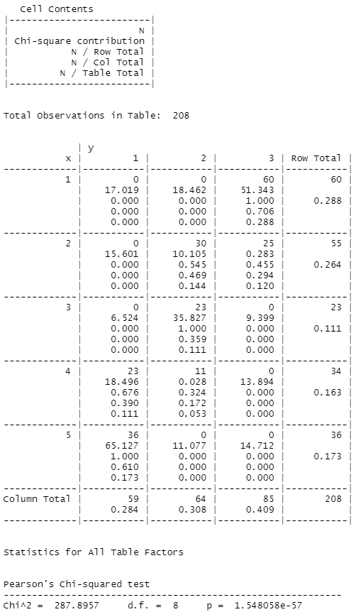 |
(5) 결과 해석
| #나이와 직위 간의 관련성이 있다를 분석하기 위해서 217명을 표본으로 추출한후 #설문조사하여 교차분석과 카이제곱검정을 시행하였다. 분석결과 나이와 직위의 #관련성은 유의미한 수준에서 차이가 있는 것으로 나타났다.(카이제곱값 = 287.8957 , p-value = 1.548058e-57 ) #따라서 귀무가설을 기각 할 수 있기때문에 나이와 직위간 관련성이 있다고 분석된다. |
4. mtcars 데이터에서 엔진(vs)을 종속변수로, 연비(mpg)와 변속기종류(am)를 독립변수로 설정하여 로지스틱 회귀분석을 실시하시오
(1) 데이터 가져오기
| data("mtcars") head(mtcars) |
(2) 로지스틱 회귀분석 실행하고 회귀모델 확인
2-1) 라이브러리
| library(car) library(lmtest) library(ROCR) |
2-2) 결측값 확인
| colSums(is.na(mtcars)) # mpg cyl disp hp drat wt qsec vs am gear carb # 0 0 0 0 0 0 0 0 0 0 0 |
2-3) 필요한 컬럼만 추출
| df<-mtcars[,c("vs","mpg","am")] |
2-4) 학습, 검증 데이터 분리
| idx <- sample(1:nrow(df), nrow(df) * 0.7) df_train <- df[idx, ] df_test <- df[-idx, ] |
2-5) 로지스틱 회귀모델 생성
| model <- glm(vs~.,data=df_train,family='binomial',na.action=na.omit) pred <- predict(model, df_test, type = "response") |
2-6) 회귀모델 예측치 생성
| result_pred <- ifelse(pred >= 0.5, 1, 0) result_pred |
2-7) 분류 정확도 계산
| table(result_pred, df_test$vs) result_pred 0 1 0 4 0 1 1 5 model # Call: glm(formula = vs ~ ., family = "binomial", data = df_train, na.action = na.omit) # # Coefficients: # (Intercept) mpg am # -10.4264 0.5619 -2.6056 # # Degrees of Freedom: 21 Total (i.e. Null); 19 Residual # Null Deviance: 29.77 # Residual Deviance: 16.24 AIC: 22.24 |
(3) 로지스틱 회귀모델 요약정보 확인
| summary(model) # Deviance Residuals: # Min 1Q Median 3Q Max # -1.8794 -0.5317 -0.2308 0.3611 1.6236 # # Coefficients: # Estimate Std. Error z value Pr(>|z|) # (Intercept) -10.4264 4.3871 -2.377 0.0175 * # mpg 0.5619 0.2513 2.236 0.0254 * # am -2.6056 1.8658 -1.396 0.1626 # --- # Signif. codes: 0 ‘***’ 0.001 ‘**’ 0.01 ‘*’ 0.05 ‘.’ 0.1 ‘ ’ 1 # # (Dispersion parameter for binomial family taken to be 1) # # Null deviance: 29.767 on 21 degrees of freedom # Residual deviance: 16.238 on 19 degrees of freedom # AIC: 22.238 # # Number of Fisher Scoring iterations: 6 |
(4) 로지스틱 회귀식
| formula(model) # vs ~ mpg + am -10.4264 + 0.5619*mpg - 2.6056*am |
(5) mpg가 30이고 자동변속기(am=0)일 때 승산(odds)?
| y = -10.4264 + 0.5619*30 - 2.6056*0 exp(y) |
5. 새롭게 제작된 자동차의 성능(주행거리(마일)/갤런)을 -30도, 0도, 30도의 기온하에 성능을 측정하였다. 각 기온당 측정된 성능데이터의 수는 4개였다. 성능데이터로부터 다음의 ANOVA 테이블을 구성하였다. 빈칸에 들어갈 숫자(정수)와 숫자를 계산한 식을 제시하시오
| Sum of Squares | Degree of Freedom | Mean Square | F | |
| Treatments | (a) | (b) | (c) | 10.8 |
| Error | (d) | (e) | 3.3334 | |
| Total | (f) | (g) |
(b):K-1 = 3-1 = 2
(e):n-k = 12-3 = 9
(g):n-1 = 12-1 = 11
(c):10.8/3.3334 = 36
(a):(b)*(c) = 2*36 = 72
(d):(e)*3.3334 = 9*3.3334 = 30
(f):(a)+(d) = 72+30 = 102
ANOVA 테이블
| Sum of Squares | Degree of Freedom | Mean Square | F | |
| Treatments | SSTR | k-1 | MSTR(=SSTR / k-1) | MSTR / MSE |
| Error | SSE | N-k | MSE(=SSE / N-k) | |
| Total | SST | N-1 |
'Q.' 카테고리의 다른 글
| [ R ] 연관분석 연습문제 (0) | 2022.12.05 |
|---|---|
| [ R ] 군집분석 연습문제 (0) | 2022.12.04 |
| [ R ] 다중회귀분석 연습문제 ch15 (0) | 2022.11.27 |
| [ R ] ch14 연습문제 (0) | 2022.11.27 |
| [ R ] 탐색적데이터 예제 평가(6) (0) | 2022.11.25 |


