
59doit
[ R ] 인공신경망 #1 본문
인공신경망(Artificial Neural Network)
- 인간의 두뇌 신경(뉴런)들이 상호작용하여 경험과 학습을 통해서 패턴을 발견하고 이를 통해서 특정 사건을 일반화하거나 데이터를 분류하는데 이용되는 기계학습방법.
- 스스로 인지하고 추론하고, 판단하여 사물을 구분하거나 인간의 개입없이 컴퓨터가 특정 상황의 미래를 예측하는데 이용될 수 있는 기계학습 방법
- 문자, 음성, 이미지 인식, 증권시장 예측, 날씨 예보 등 다양한 분야에서 활용.
- 활성함수
활성 함수는 망의 총합과 경계값(bias)를 계산하여 출력신호(y)를 결정 일반적으로 활성 함수는 0과 1사이의 확률분포를 갖는 시그모이드 함수(Sigmoid function)를 이용 현재 인공신경망에서는 시그모이드 함수를 이용한다
- 퍼셉트론(Perceptron)
생물학적인 신경망처럼 신경과 신경이 하나의 망 형태로 나타내기 위해서 여러 개의 계층으로 다층화하여 만들어진 인공신경망.
- 인공신경망 기계학습과 역전파 알고리즘
출력값(o1)과 실제 관측값(y1)을 비교하여 오차(E)를 계산하고, 이러한 오차(E)를 줄이기 위해서 가중치(w)와 경계값(b)를 조정한다.
오차(E) = 관측값(y1) – 출력값(o1) 인공신경망(퍼셉트론)은 기본적으로 단방향 망(Feed Forward Network)으로 구성된다.
즉 입력측 → 은닉층 → 출력층의 한 방향으로만 전파되는데 이런 전파 방식을 개선하여 역방향으로 오차를 전파하여 은닉층의 가중치와 경계값을 조정하여 분류정확도를 높이는 역전파(Backpropagation) 알고리즘을 도입.
역전파 알고리즘은 출력에서 생긴 오차를 신경망의 역방향(입력층)으로 전파하여 순차적으로 편미분을 수행하면서 가중치(w)와 경계값(b)등을 수정한다.
ex ) 간단한 인공신경망 모델 생성
nnet패키지에서 제공하는 nnet()함수 : nnet(formula, data, weights, size)
- formula: y ~ x 형식으로 반응변수와 설명변수 식
- data: 모델 생성에 사용될 데이터 셋
- weights: 각 case에 적용할 가중치(기본값: 1)
- size: 은닉층(hidden layer)의 수 지정
#1 패키지 설치
| install.packages("nnet") library(nnet) |
#2 데이터 셋 생성
| df = data.frame( x2 = c(1:6), x1 = c(6:1), y = factor(c('no', 'no', 'no', 'yes', 'yes', 'yes')) ) str(df) # 'data.frame': 6 obs. of 3 variables: # $ x2: int 1 2 3 4 5 6 # $ x1: int 6 5 4 3 2 1 # $ y : Factor w/ 2 levels "no","yes": 1 1 1 2 2 2 |
#3 인공신경망 모델 생성
| model_net=nnet(y~.,df,size=1) # weights: 5 # initial value 3.816777 # iter 10 value 0.011575 # final value 0.000079 # converged |
- size : 은닉층 수
#4 모델 결과 변수 보기
| model_net # a 2-1-1 network with 5 weights # inputs: x2 x1 # output(s): y # options were - entropy fitting |
#5 가중치(weights)보기
| summary(model_net) # a 2-1-1 network with 5 weights # options were - entropy fitting # b->h1 i1->h1 i2->h1 # -0.34 8.66 -8.52 # b->o h1->o # -10.76 22.9 |
#6 분류모델의 적합값 보기
| model_net$fitted.values # [,1] # 1 2.116418e-05 # 2 2.116418e-05 # 3 2.126881e-05 # 4 9.999948e-01 # 5 9.999948e-01 # 6 9.999948e-01 |
df # x2 x1 y # 1 1 6 no # 2 2 5 no # 3 3 4 no # 4 4 3 yes # 5 5 2 yes # 6 6 1 yes |
$fitted.values ??
| str(model_net) # List of 19 # $ n : num [1:3] 2 1 1 # $ nunits : int 5 # $ nconn : num [1:6] 0 0 0 0 3 5 # $ conn : num [1:5] 0 1 2 0 3 # $ nsunits : int 5 # $ decay : num 0 # $ entropy : logi TRUE # $ softmax : logi FALSE # $ censored : logi FALSE # $ value : num 7.92e-05 # $ wts : num [1:5] -0.337 8.659 -8.521 -10.763 22.929 # $ convergence : int 0 # $ fitted.values: num [1:6, 1] 2.12e-05 2.12e-05 2.13e-05 1.00 1.00 ... # ..- attr(*, "dimnames")=List of 2 # .. ..$ : chr [1:6] "1" "2" "3" "4" ... # .. ..$ : NULL # $ residuals : num [1:6, 1] -2.12e-05 -2.12e-05 -2.13e-05 5.23e-06 5.21e-06 ... # ..- attr(*, "dimnames")=List of 2 # .. ..$ : chr [1:6] "1" "2" "3" "4" ... # .. ..$ : NULL # $ lev : chr [1:2] "no" "yes" # $ call : language nnet.formula(formula = y ~ ., data = df, size = 1) # $ terms :Classes 'terms', 'formula' language y ~ x2 + x1 # .. ..- attr(*, "variables")= language list(y, x2, x1) # .. ..- attr(*, "factors")= int [1:3, 1:2] 0 1 0 0 0 1 # .. .. ..- attr(*, "dimnames")=List of 2 # .. .. .. ..$ : chr [1:3] "y" "x2" "x1" # .. .. .. ..$ : chr [1:2] "x2" "x1" # .. ..- attr(*, "term.labels")= chr [1:2] "x2" "x1" # .. ..- attr(*, "order")= int [1:2] 1 1 # .. ..- attr(*, "intercept")= int 1 # .. ..- attr(*, "response")= int 1 # .. ..- attr(*, ".Environment")=<environment: R_GlobalEnv> # .. ..- attr(*, "predvars")= language list(y, x2, x1) # .. ..- attr(*, "dataClasses")= Named chr [1:3] "factor" "numeric" "numeric" # .. .. ..- attr(*, "names")= chr [1:3] "y" "x2" "x1" # $ coefnames : chr [1:2] "x2" "x1" # $ xlevels : Named list() # - attr(*, "class")= chr [1:2] "nnet.formula" "nnet" |
model_net 의 구조를 보면 여러 가지 value가 나오는데
nnet function - RDocumentation
nnet(x, …) # S3 method for formula nnet(formula, data, weights, …, subset, na.action, contrasts = NULL) # S3 method for default nnet(x, y, weights, size, Wts, mask, linout = FALSE, entropy = FALSE, softmax = FALSE, censored = FALSE, skip = FALSE, rang
www.rdocumentation.org
사이트에서
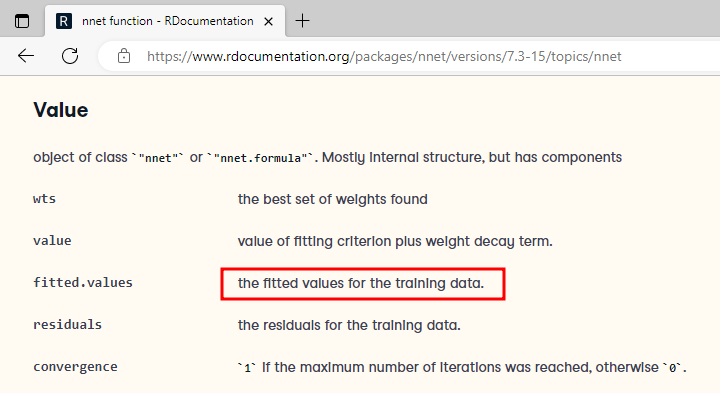
보면 fitted.values 가 학습 데이터에 대한 적합치를 볼 수 있는 value로 설명되어있음을 알 수 있다.
따라서 model_net$fitted.values 를 사용 하였다.
#7 분류모델의 예측치 생성과 분류 정확도
| p <- predict(model_net,df,type="class") table(p,df$y) # p no yes # no 3 0 # yes 0 3 |
p <- predict(model_net,df,type="raw") table(p,df$y) # p no yes # 2.11641831645402e-05 2 0 # 2.12688051032348e-05 1 0 # 0.999994774896315 0 1 # 0.999994794118989 0 2 |
||
type="class" ??

nnet에서 type(출력유형은) raw, class를 사용한다
위에서 분류정확도를 보기위해 사용한 출력유형을 두가지 경우로 제시해 보았다.
ex ) iris 데이터 셋을 이용한 인공신경망 모델 생성
#1 데이터 생성
| data(iris) idx = sample(1:nrow(iris), 0.7 * nrow(iris)) training = iris[idx, ] testing = iris[-idx, ] nrow(training) # [1] 105 nrow(testing) # [1] 45 |
#2 인공신경망 모델(은닉층 1개와 은닉층 3개) 생성
| iris # Sepal.Length Sepal.Width Petal.Length Petal.Width Species # 1 5.1 3.5 1.4 0.2 setosa # 2 4.9 3.0 1.4 0.2 setosa # 3 4.7 3.2 1.3 0.2 setosa # 4 4.6 3.1 1.5 0.2 setosa # 5 5.0 3.6 1.4 0.2 setosa |
| model_net_iris1=nnet(Species ~ ., training,size=1) # # weights: 11 # initial value 131.949452 # final value 115.239942 # converged model_net_iris1 # a 4-1-3 network with 11 weights # inputs: Sepal.Length Sepal.Width Petal.Length Petal.Width # output(s): Species # options were - softmax modelling model_net_iris3=nnet(Species ~ ., training,size=3) # # weights: 27 # initial value 135.486282 # iter 10 value 41.163797 # iter 20 value 11.982971 # iter 30 value 10.049970 # iter 40 value 6.301342 # iter 50 value 3.467637 # iter 60 value 0.866640 # iter 70 value 0.045099 # iter 80 value 0.000540 # iter 90 value 0.000258 # final value 0.000060 # converged model_net_iris3 # a 4-3-3 network with 27 weights # inputs: Sepal.Length Sepal.Width Petal.Length Petal.Width # output(s): Species # options were - softmax modelling |
입력 변수의 갑들이 일정하지 않거나 값이 큰 경우에는 신경망 모델이 정상적으로 만들어지지 않기 때문에 입력 변수를 대상으로 정규화 과정이 필요하다.
#3 가중치 네트워크 보기 – 은닉층 1개 신경망 모델
| summary(model_net_iris1) # a 4-1-3 network with 11 weights # options were - softmax modelling # b->h1 i1->h1 i2->h1 i3->h1 i4->h1 # 0.00 -1.80 -1.89 -0.21 -0.20 # b->o1 h1->o1 # 0.23 0.03 # b->o2 h1->o2 # 0.29 0.28 # b->o3 h1->o3 # 0.34 -0.09 |
#4 가중치 네트워크 보기 – 은닉층 3개 신경망 모델
| summary(model_net_iris3) # a 4-3-3 network with 27 weights # options were - softmax modelling # b->h1 i1->h1 i2->h1 i3->h1 i4->h1 # 417.22 -8.08 144.14 -0.65 -443.48 # b->h2 i1->h2 i2->h2 i3->h2 i4->h2 # -6.76 0.23 -0.58 2.74 -3.30 # b->h3 i1->h3 i2->h3 i3->h3 i4->h3 # -2.10 -7.52 -3.86 -3.05 -1.34 # b->o1 h1->o1 h2->o1 h3->o1 # 116.72 141.93 -713.57 0.78 # b->o2 h1->o2 h2->o2 h3->o2 # -62.54 207.51 40.82 2.82 # b->o3 h1->o3 h2->o3 h3->o3 # -54.48 -350.20 673.60 -3.93 |
#5 분류모델 평가
| table(predict(model_net_iris1,testing,type="class"),testing$Species) # setosa versicolor virginica # virginica 17 15 13 table(predict(model_net_iris3,testing,type="class"),testing$Species) # setosa versicolor virginica # setosa 17 1 0 # versicolor 0 13 0 # virginica 0 1 13 |
- classificationMetrics() 함수: 분류 metrics 생성
'통계기반 데이터분석' 카테고리의 다른 글
| [ R ] 서포트벡터머신 (SVM) (0) | 2022.12.01 |
|---|---|
| [ R ] 인공신경망 #2 neuralnet 패키지이용 (0) | 2022.12.01 |
| [ R ] 앙상블 #2 - 랜덤포레스트 예제 (0) | 2022.11.30 |
| [ R ] 앙상블 #1 - 배깅 & 부스팅 & 랜덤포레스트 (0) | 2022.11.30 |
| [ R ] 의사결정나무 #4 rpart패키지 이용 분류분석 (0) | 2022.11.29 |


