
59doit
[ R ] 앙상블 #1 - 배깅 & 부스팅 & 랜덤포레스트 본문
앙상블(Ensemble)
의사결정나무의 문제점을 ctree와 다른 방식으로 보완하기 위하여 개발된 방법
주어진 자료로부터 예측 모형을 여러 개 만들고, 이것을 결합하여 최종적인 예측 모형을 만드는 방법
배깅(Breiman, 1996) → 부스팅 개발 → 랜덤포레스트(Random Forest)
앙상블에서 사용되는 기법: 배깅, 부스팅, 랜덤포레스트
1. 배깅(Bagging)
- 불안정한 예측모형에서 불안정성을 제거함으로써 예측력을 향상
- 불안정한 예측모형: 데이터의 작은 변화에도 예측 모형이 크게 바뀌는 경우
- Bootstrap AGGregatING의 준말
- 주어진 자료에 대하여 여러 개의 부트스트랩(bootstrap)자료를 만들고, 각 부트스트랩 자료에 예측 모형을 만든 다음, 이것을 결합하여 최종 예측 모형을 만드는 방법
- 부트스트랩자료: 주어진 자료로부터 동일한 크기의 표본을 랜덤 복원 추출로 뽑은 것
# 1 패키지 및 라이브러리
| install.packages("party") install.packages("caret") library(party) library(caret) |
# 2 data sampling
| data1 <- iris[sample(1:nrow(iris), replace=T),] data2 <- iris[sample(1:nrow(iris), replace=T),] data3 <- iris[sample(1:nrow(iris), replace=T),] data4 <- iris[sample(1:nrow(iris), replace=T),] data5 <- iris[sample(1:nrow(iris), replace=T),] |
# 3 예측모형 생성
| citree1 <- ctree(Species~., data1) citree2 <- ctree(Species~., data2) citree3 <- ctree(Species~., data3) citree4 <- ctree(Species~., data4) citree5 <- ctree(Species~., data5) |
# 4 예측수행
| predicted1 <- predict(citree1, iris) predicted2 <- predict(citree2, iris) predicted3 <- predict(citree3, iris) predicted4 <- predict(citree4, iris) predicted5 <- predict(citree5, iris) |
# 5 예측모형 결합하여 새로운 예측모형 생성
| newmodel <- data.frame(Species=iris$Species, predicted1,predicted2,predicted3,predicted4,predicted5) head(newmodel) # Species predicted1 predicted2 predicted3 predicted4 predicted5 # 1 setosa setosa setosa setosa setosa setosa # 2 setosa setosa setosa setosa setosa setosa # 3 setosa setosa setosa setosa setosa setosa # 4 setosa setosa setosa setosa setosa setosa # 5 setosa setosa setosa setosa setosa setosa # 6 setosa setosa setosa setosa setosa setosa newmodel |
# 6 최종모형으로 통합
| funcValue <- function(x) { result <- NULL for(i in 1:nrow(x)) { xtab <- table(t(x[i,])) rvalue <- names(sort(xtab, decreasing = T) [1]) result <- c(result,rvalue) } return (result) } newmodel |
# 7 최종 모형의 2번째에서 6번째를 통합하여 최종 결과 생성
| newmodel$result <- funcValue(newmodel[, 2:6]) newmodel$result |
# 8 최종결과 비교
| table(newmodel$result, newmodel$Species) # setosa versicolor virginica # setosa 50 0 0 # versicolor 0 48 4 # virginica 0 2 46 |
2. 부스팅(Boosting)
예측력이 약한 모형만 만들어지는 경우, 예측력이 약한 모형들을 결합하여 강한 예측모형을 만드는 방법
예측력이 약한 모형: 랜덤하게 예측하는 것보다 더 좋은 예측력을 가진 모형
3. 랜덤포레스트(Random Forest)
- 2001년 Breiman에 의해 개발.
- 배깅과 부스팅보다 더 많은 무작위성을 주어서 약한 학습 모델을 만든 다음, 이것을 선형 결합하여 최종학습기를 만드는 방법
- 예측력이 매우 높음.
- 입력 변수 개수가 많을 때는 배깅이나 부스팅과 비슷하거나 더 좋은 예측력을 보여주어 많이 사용된다.
- 랜덤포레스트 방식은 기존의 의사결정 트리 방식에 비해서 많은 데이터를 이용하여 학습을 수행하기 때문에 비교적 예측력이 뛰어나고, 과적합(overfitting)문제를 해결할 수 있다.
- 랜덤포레스트 모델은 기본적으로 원 데이터(raw data)를 대상으로 복원추출 방식으로 데이터의 양을 증가시킨 후 모델을 생성하기 때문에 데이터의 양이 부족해서 발생하는 과적합의 원인을 해결할 수 있다.
- 각각의 분류모델에서 예측된 결과를 토대로 투표방식(voting)으로 최적의 예측치 선택
# 1 iris 데이터
| data(iris) head(iris) |
# 2 70% training데이터, 30% testing데이터로 구분
| idx <- sample(2, nrow(iris), replace=T, prob=c(0.7, 0.3)) trainData <- iris[idx == 1, ] testData <- iris[idx == 2, ] |
# 3 랜덤 포레스트 라이브러리
| library(randomForest) |
# 4 랜덤포레스트 실행 (100개의 tree를 다양한 방법(proximity=T)으로 생성)
| RFmodel <- randomForest(Species~., data=trainData, ntree=100, proximity=T) RFmodel # Call: # randomForest(formula = Species ~ ., data = trainData, ntree = 100, proximity = T) # Type of random forest: classification # Number of trees: 100 # No. of variables tried at each split: 2 # # OOB estimate of error rate: 4.76% # Confusion matrix: # setosa versicolor virginica class.error # setosa 37 0 0 0.00000000 # versicolor 0 28 3 0.09677419 # virginica 0 2 35 0.05405405 |
# 5 시각화
plot(RFmodel, main="RandomForest Model of iris")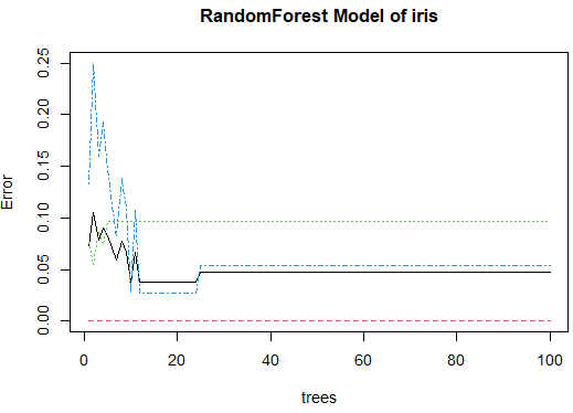 |
# 6 모델에 사용된 변수 중 중요한 것 확인
| importance(RFmodel) # MeanDecreaseGini # Sepal.Length 8.473552 # Sepal.Width 1.991675 # Petal.Length 31.467776 # Petal.Width 27.174711 |
# 7 중요한 것 시각화
varImpPlot(RFmodel)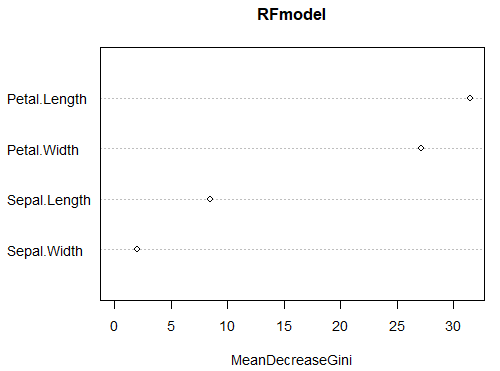 |
# 8 실제값과 예측값 비교
| table(trainData$Species, predict(RFmodel)) # setosa versicolor virginica # setosa 37 0 0 # versicolor 0 28 3 # virginica 0 2 35 |
# 9 테스트데이터로 예측
| pred <- predict(RFmodel, newdata=testData) |
# 10 실제값과 예측값 비교
| table(testData$Species, pred) # pred # setosa versicolor virginica # setosa 13 0 0 # versicolor 0 17 2 # virginica 0 0 13 |
# 11 시각화
plot(margin(RFmodel, testData$Species))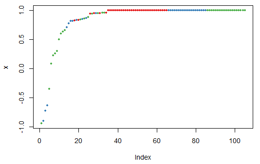 |
그래프에서 모델 오류가 안정적인 상태를 보이기 시작하는 시점의 tree개수로 실행
< 중요한 것 시각화 ? >
varImpPlot(RFmodel)의 그래프에서 Petal.Width, Petal.Length가 중요변수
'통계기반 데이터분석' 카테고리의 다른 글
| [ R ] 인공신경망 #1 (0) | 2022.12.01 |
|---|---|
| [ R ] 앙상블 #2 - 랜덤포레스트 예제 (0) | 2022.11.30 |
| [ R ] 의사결정나무 #4 rpart패키지 이용 분류분석 (0) | 2022.11.29 |
| [ R ] 의사결정나무 조건부 추론나무 #3 예제 (0) | 2022.11.29 |
| [ R ] 의사결정나무 #2 (0) | 2022.11.29 |


