
59doit
[ R ] 의사결정나무 #1 본문
의사결정나무
CART(Classification and Regression Tree) : 가장 많이 쓰는 기법
C4.5 & C5.0 : CART와 다르게 node에서 다지분리(Multiple Split)이 가능
CHAID(Chi-squared Automatic Interaction Detection) : 범주형 변수에 적용 가능
1. 의사결정 트리(Decision Tree)
의사결정트리 방식은 나무(Tree)구조 형태로 분류 결과를 도출
(1) party 패키지 이용 분류분석
조건부 추론 나무
CART기법으로 구현한 의사결정나무의 문제점
1) 통계적 유의성에 대한 판단없이 노드를 분할하는데 대한 과적합(Overfitting) 발생 문제.
2) 다양한 값으로 분할 가능한 변수가 다른 변수에 비해 선호되는 현상
이 문제점을 해결하는 조건부 추론 나무(Conditional Inference Tree).
party패키지의 ctree()함수 이용
의사결정 트리 생성: ctree()함수 이용
#1 party패키지 설치
| install.packages("party") library(party) |
#2 airquality 데이터셋 로딩
| library(datasets) str(airquality) # 'data.frame': 153 obs. of 6 variables: # $ Ozone : int 41 36 12 18 NA 28 23 19 8 NA ... # $ Solar.R: int 190 118 149 313 NA NA 299 99 19 194 ... # $ Wind : num 7.4 8 12.6 11.5 14.3 14.9 8.6 13.8 20.1 8.6 ... # $ Temp : int 67 72 74 62 56 66 65 59 61 69 ... # $ Month : int 5 5 5 5 5 5 5 5 5 5 ... # $ Day : int 1 2 3 4 5 6 7 8 9 10 ... |
#3 formula생성
| formula <- Temp ~ Solar.R + Wind + Ozone |
formula?
#4 분류모델 생성 – formula를 이용하여 분류모델 생성
| air_ctree <- ctree(formula, data = airquality) air_ctree # Conditional inference tree with 5 terminal nodes # # Response: Temp # Inputs: Solar.R, Wind, Ozone # Number of observations: 153 # # 1) Ozone <= 37; criterion = 1, statistic = 56.086 # 2) Wind <= 15.5; criterion = 0.993, statistic = 9.387 # 3) Ozone <= 19; criterion = 0.964, statistic = 6.299 # 4)* weights = 29 # 3) Ozone > 19 # 5)* weights = 69 # 2) Wind > 15.5 # 6)* weights = 7 # 1) Ozone > 37 # 7) Ozone <= 65; criterion = 0.971, statistic = 6.691 # 8)* weights = 22 # 7) Ozone > 65 # 9)* weights = 26 |
첫번째: 반응변수(종속변수)에 대해서 설명변수(독립변수)가 영향을 미치는 중요 변수의 척도. 수치가 작을수록 영향을 미치는 정도가 높고, 순서는 분기되는 순서를 의미
두번째: 의사결정 트리의 노드명
세번째: 노드이 분기기준(criterion)이 되는 수치.
네번째: 반응변수(종속변수)의 통계량(statistic). *마지막 노드이거나 또 다른 분기 기준이 있는 경우에는 세번째와 네 번째 수치는 표시되지 않는다.
#5 분류분석 결과 plot(air_ctree)
plot(air_ctree)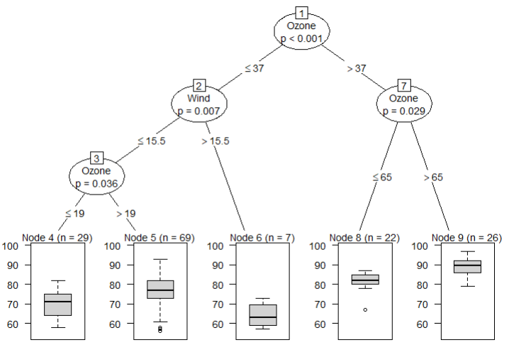 |
학습데이터와 검정데이터 샘플링으로 분류분석 수행
#1 학습데이터와 검정데이터 샘플링 ( iris 데이터 이용 )
| set.seed(1234) idx <- sample(1:nrow(iris), nrow(iris) * 0.7) train <- iris[idx, ] test <- iris[-idx, ] |
#2 formula생성
| formula <- Species ~ Sepal.Length + Sepal.Width + Petal.Length + Petal.Width |
#3 학습데이터 이용 분류모델 생성
| iris_ctree <- ctree(formula, data = train) iris_ctree # Conditional inference tree with 4 terminal nodes # # Response: Species # Inputs: Sepal.Length, Sepal.Width, Petal.Length, Petal.Width # Number of observations: 105 # # 1) Petal.Length <= 1.9; criterion = 1, statistic = 98.365 # 2)* weights = 34 # 1) Petal.Length > 1.9 # 3) Petal.Width <= 1.6; criterion = 1, statistic = 47.003 # 4) Petal.Length <= 4.6; criterion = 1, statistic = 14.982 # 5)* weights = 28 # 4) Petal.Length > 4.6 # 6)* weights = 8 # 3) Petal.Width > 1.6 # 7)* weights = 35 |
#4 분류모델 플로팅
4-1) 간단한 형식으로 시각화
plot(iris_ctree, type = "simple")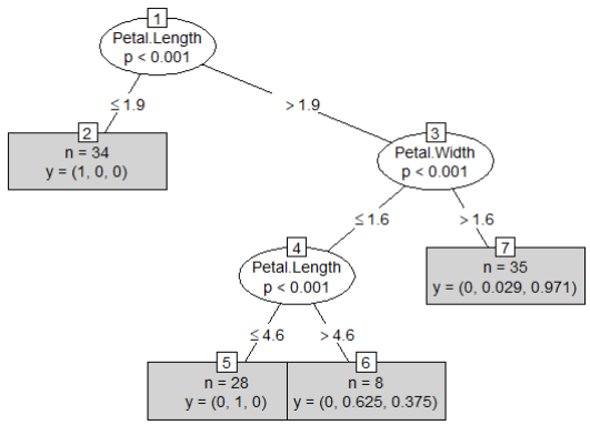 |
4-2) 의사결정 트리로 결과 플로팅
plot(iris_ctree)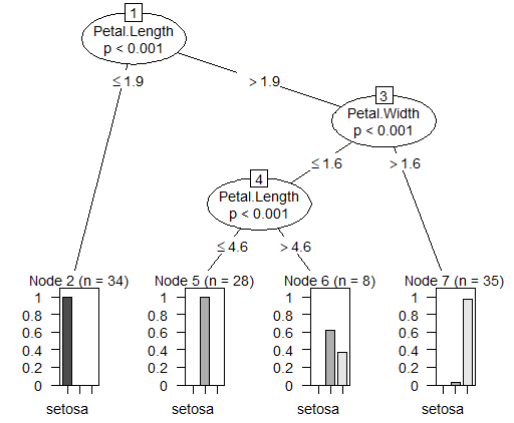 |
#5 분류모델 평가
#5-1)모델의 예측치 생성과 혼돈 매트릭스 생성
| pred <- predict(iris_ctree, test) table(pred, test$Species) # pred setosa versicolor virginica # setosa 16 0 0 # versicolor 0 15 1 # virginica 0 1 12 |
5-2) 분류 정확도
| (14 + 16 + 13) / nrow(test) | caret::confusionMatrix(test$Species, pred)$overall[1] |
동일한 결과
Accuracy
0.9555556
caret::confusionMatrix(테스트데이터, 예측데이터)$overall[1]
'통계기반 데이터분석' 카테고리의 다른 글
| [ R ] 의사결정나무 조건부 추론나무 #3 예제 (0) | 2022.11.29 |
|---|---|
| [ R ] 의사결정나무 #2 (0) | 2022.11.29 |
| [ R ] 시계열분석 #2 (0) | 2022.11.28 |
| [ R ] 시계열분석 #1 (1) | 2022.11.28 |
| [ R ] 로지스틱 회귀분석 (0) | 2022.11.28 |


