
59doit
[ R ] 다양한 시각화 #2 점 ㆍ산점도 그래프 본문
(4) 점 그래프
dotplot()함수 : dotplot(y축 컬럼 ~ x축 컬럼 |조건, data. layout)
# dotplot()함수를 사용하여 점 그래프 그리기
#1 layout 속성이 없는 경우
dotplot(Var1~Freq|Var2,dft) |
#2 layout 속성 적용한 경우
dotplot(Var1~Freq|Var2,dft,layout=c(4,1)) |
# 점을 선으로 연결하여 시각화히기
| dotplot(Var1~Freq,data=dft, groups=Var2, type = "O", auto.key=list(space="rigth", points=T, lines=T)) |
영어 알파벳 O, 숫자0아니다
- type='O': 점(point)타입으로 원형에 실선이 통과하는 유형으로 그래프의 타입을 지정
- auto.key=list(space=”right”, points=T, lines=T): 범례를 타나내는 속성. 범례의 위치는 오른쪽으로 지정, 점과 선을 범례에 표시
(5) 산점도 그래프
xyplot()함수 : xyplot(y축 컬럼 ~ x축 컬럼|조건변수, data=data.frame 또는 list, layout)
# airquality 데이터 셋으로 산점도 그래프 그리기
#1 데이터 가져오기 ( airquality 이용 )
| library(datasets) str(airquality) head(airquality) # Ozone Solar.R Wind Temp Month Day # 1 41 190 7.4 67 5 1 # 2 36 118 8.0 72 5 2 # 3 12 149 12.6 74 5 3 # 4 18 313 11.5 62 5 4 # 5 NA NA 14.3 56 5 5 # 6 28 NA 14.9 66 5 6 |
#2 xyplot()함수를 사용하여 산점도 그리기
xyplot(Ozone~Wind, data=airquality) |
#3 조건변수를 사용하는 xyplot()함수로 산점도 그리기
xyplot(Ozone~Wind|Month,data=airquality,layout=c(5,1)) |
#4 조건변수+layout 사용 하여 산점도 그리기
xyplot(Ozone~Wind|Month,data=airquality,layout=c(5,1)) |
#5 변수를 factor타입으로 변환하여 산점도 그리기 (패널 제목에는 factor값을 표시)
| convert <- transform(airquality,Month=factor(Month)) str(convert) 'data.frame': 153 obs. of 6 variables: $ Ozone : int 41 36 12 18 NA 28 23 19 8 NA ... $ Solar.R: int 190 118 149 313 NA NA 299 99 19 194 ... $ Wind : num 7.4 8 12.6 11.5 14.3 14.9 8.6 13.8 20.1 8.6 ... $ Temp : int 67 72 74 62 56 66 65 59 61 69 ... $ Month : Factor w/ 5 levels "5","6","7","8",..: 1 1 1 1 1 1 1 1 1 1 ... $ Day : int 1 2 3 4 5 6 7 8 9 10 ... xyplot(Ozone~Wind|Month,data=convert)  xyplot(Ozone~Wind|Month,data=convert,layout=c(5,1)) 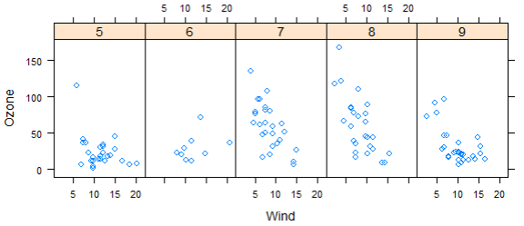 |
# quakes 데이터 셋으로 산점도 그래프 그리기
#1 데이터 가져오기 ( quakes 이용 ) quakes : 지질
| head(quakes) # lat long depth mag stations depth2 depth3 mag3 # 1 -20.42 181.62 562 4.8 41 6 d4 m2 # 2 -20.62 181.03 650 4.2 15 6 d5 m1 # 3 -26.00 184.10 42 5.4 43 1 d1 m2 # 4 -17.97 181.66 626 4.1 19 6 d5 m1 # 5 -20.42 181.96 649 4.0 11 6 d5 m1 # 6 -19.68 184.31 195 4.0 12 2 d3 m1 str(quakes) # 'data.frame': 1000 obs. of 8 variables: # $ lat : num -20.4 -20.6 -26 -18 -20.4 ... # $ long : num 182 181 184 182 182 ... # $ depth : int 562 650 42 626 649 195 82 194 211 622 ... # $ mag : num 4.8 4.2 5.4 4.1 4 4 4.8 4.4 4.7 4.3 ... # $ stations: int 41 15 43 19 11 12 43 15 35 19 ... # $ depth2 : num 6 6 1 6 6 2 1 2 2 6 ... # $ depth3 : chr "d4" "d5" "d1" "d5" ... # $ mag3 : chr "m2" "m1" "m2" "m1" ... |
#2 지진 발생 진앙지(위도, 경도) 산점도 그리기
xyplot(lat~long, data=quakes,pch=".") |
발생한 위치가 점(.) 으로 산점도 표현
#3 산점도 그래프를 변수에 저장하고, 제목 문자열 추가하기
| tplot <- xyplot(lat~long,data=quakes, pch=".") # 산점도 그래프를 tplot에 저장 tplot <- update(tplot, main = "1964년 이후 태평양에서 발생한 지진 위치") # 제목 문자열 추가하기 print(tplot)  |
# 이산형 변수를 조건으로 지정하여 산점도 그리기
수심별로 진앙지를 파악하기 위해서 depth변수를 조건으로 지정
#1 depth 변수의 범위 확인
| range(quakes$depth) # 40 680 |
#2 depth 변수 리코딩 : 6개의 범주로 코딩 변경 (100단위)
| quakes$depth2[quakes$depth >= 40 & quakes$depth <= 150] <- 1 quakes$depth2[quakes$depth >= 151 & quakes$depth <= 250] <- 2 quakes$depth2[quakes$depth >= 251 & quakes$depth <= 350] <- 3 quakes$depth2[quakes$depth >= 351 & quakes$depth <= 450] <- 4 quakes$depth2[quakes$depth >= 451 & quakes$depth <= 550] <- 5 quakes$depth2[quakes$depth >= 551 & quakes$depth <= 680] <- 6 |
#3 depth2조건으로 산점도 그리기
| convert <- transform(quakes,depth2=factor(depth2)) xyplot(lat~long|depth2,data=convert)  |
# 동일한 패널에 두 개의 변수값 표현하기
#1 동일한 패널에 두개의 변수값 표현하기
| head(airquality) # Ozone Solar.R Wind Temp Month Day # 1 41 190 7.4 67 5 1 # 2 36 118 8.0 72 5 2 # 3 12 149 12.6 74 5 3 # 4 18 313 11.5 62 5 4 # 5 NA NA 14.3 56 5 5 # 6 28 NA 14.9 66 5 6 |
#2 depth 변수 리코딩 : 6개의 범주로 코딩 변경 (100단위)
| xyplot(Ozone + Solar.R ~ Wind|factor(Month), data=airquality, col=c("blue","red"), layout=c(5,1))  |
Ozone : y1축
Solar.R : y2축
Wind : x축
month : 조건 (factor형으로 변환)
'Programming > R' 카테고리의 다른 글
| [ R ]다양한 시각화 # 4 조건 그래프 (0) | 2022.12.23 |
|---|---|
| [ R ]다양한 시각화 # 3 데이터범주화 (0) | 2022.12.23 |
| [ R ] 다양한 시각화 #1 히스토그램 밀도ㆍ막대 그래프 (0) | 2022.12.23 |
| [ R ] 데이터 시각화 #2 연속변수 시각화 (2) (1) | 2022.12.22 |
| [ R ] 데이터 시각화 #2 연속변수 시각화 (1) (0) | 2022.12.22 |


