
59doit
[ R ] 연관분석 #2 시각화 본문
(3) 연관규칙 시각화
arules패키지에서 제공되는 내장 데이터 Adult를 이용하여 연관규칙을 생성하고 유사한 연관규칙끼리 네트워크 형태로 시각화
연관분석과 관련된 패키지를 가지고 있음
ex) Adult 데이터 셋 가져오기
| data(Adult) Adult # transactions in sparse format with # 48842 transactions (rows) and # 115 items (columns) |
ex) AdultUCI 데이터 셋 보기
| data("AdultUCI") str(AdultUCI) |
ex) Adult 데이터 셋의 요약통계량 보기
#1 data.frame형식으로 보기
| adult <- as(Adult, "data.frame") str(adult) head(adult) |
#2 요약통계량
| summary(Adult) |
ex) 지지도 10%와 신뢰도 80%가 적용된 연관규칙 발견 6137개
| ar <- apriori(Adult, parameter = list(supp = 0.1, conf = 0.8)) # Apriori # # Parameter specification: # confidence minval smax arem aval originalSupport maxtime support minlen maxlen target ext # 0.8 0.1 1 none FALSE TRUE 5 0.1 1 10 rules TRUE # # Algorithmic control: # filter tree heap memopt load sort verbose # 0.1 TRUE TRUE FALSE TRUE 2 TRUE # # Absolute minimum support count: 4884 # # set item appearances ...[0 item(s)] done [0.00s]. # set transactions ...[115 item(s), 48842 transaction(s)] done [0.04s]. # sorting and recoding items ... [31 item(s)] done [0.01s]. # creating transaction tree ... done [0.03s]. # checking subsets of size 1 2 3 4 5 6 7 8 9 done [0.11s]. # writing ... [6137 rule(s)] done [0.01s]. # creating S4 object ... done [0.01s]. |
ex) 다양한 신뢰도와 지지도를 적용한 예
#1 지지도를 20%로 높인 경우 1,306개 규칙 발견
| ar1 <- apriori(Adult, parameter = list(supp = 0.2)) # Parameter specification: # confidence minval smax arem aval originalSupport maxtime support minlen maxlen target # 0.8 0.1 1 none FALSE TRUE 5 0.2 1 10 rules # ext # TRUE # # Algorithmic control: # filter tree heap memopt load sort verbose # 0.1 TRUE TRUE FALSE TRUE 2 TRUE # # Absolute minimum support count: 9768 # # set item appearances ...[0 item(s)] done [0.00s]. # set transactions ...[115 item(s), 48842 transaction(s)] done [0.04s]. # sorting and recoding items ... [18 item(s)] done [0.01s]. # creating transaction tree ... done [0.02s]. # checking subsets of size 1 2 3 4 5 6 7 done [0.01s]. # writing ... [1306 rule(s)] done [0.00s]. # creating S4 object ... done [0.00s]. |
#2 지지도를 20%, 신뢰도 95%로 높인 경우 348개 규칙 발견 (#1 에서 신뢰도를 더 높임)
| ar1 <- apriori(Adult, parameter = list(supp = 0.2, conf = 0.95 )) # Apriori # # Parameter specification: # confidence minval smax arem aval originalSupport maxtime support minlen maxlen target # 0.95 0.1 1 none FALSE TRUE 5 0.2 1 10 rules # ext # TRUE # # Algorithmic control: # filter tree heap memopt load sort verbose # 0.1 TRUE TRUE FALSE TRUE 2 TRUE # # Absolute minimum support count: 9768 # # set item appearances ...[0 item(s)] done [0.00s]. # set transactions ...[115 item(s), 48842 transaction(s)] done [0.04s]. # sorting and recoding items ... [18 item(s)] done [0.01s]. # creating transaction tree ... done [0.03s]. # checking subsets of size 1 2 3 4 5 6 7 done [0.01s]. # writing ... [348 rule(s)] done [0.00s]. # creating S4 object ... done [0.00s]. |
#3 지지도를 30%, 신뢰도 95%로 높인 경우 124개 규칙 발견 (#2 에서 지지도를 더 높임)
| ar3 <- apriori(Adult, parameter = list(supp = 0.3, conf = 0.95)) # Apriori # # Parameter specification: # confidence minval smax arem aval originalSupport maxtime support minlen maxlen target # 0.95 0.1 1 none FALSE TRUE 5 0.3 1 10 rules # ext # TRUE # # Algorithmic control: # filter tree heap memopt load sort verbose # 0.1 TRUE TRUE FALSE TRUE 2 TRUE # # Absolute minimum support count: 14652 # # set item appearances ...[0 item(s)] done [0.00s]. # set transactions ...[115 item(s), 48842 transaction(s)] done [0.04s]. # sorting and recoding items ... [14 item(s)] done [0.01s]. # creating transaction tree ... done [0.03s]. # checking subsets of size 1 2 3 4 5 6 done [0.00s]. # writing ... [124 rule(s)] done [0.00s]. # creating S4 object ... done [0.00s]. |
#4 지지도를 35%, 신뢰도 95%로 높인 경우 67개 규칙 발견 (#3 에서 지지도를 더 높임)
| ar4 <- apriori(Adult, parameter = list(supp = 0.35, conf = 0.95)) # Apriori # # Parameter specification: # confidence minval smax arem aval originalSupport maxtime support minlen maxlen target # 0.95 0.1 1 none FALSE TRUE 5 0.35 1 10 rules # ext # TRUE # # Algorithmic control: # filter tree heap memopt load sort verbose # 0.1 TRUE TRUE FALSE TRUE 2 TRUE # # Absolute minimum support count: 17094 # # set item appearances ...[0 item(s)] done [0.00s]. # set transactions ...[115 item(s), 48842 transaction(s)] done [0.04s]. # sorting and recoding items ... [11 item(s)] done [0.01s]. # creating transaction tree ... done [0.03s]. # checking subsets of size 1 2 3 4 5 done [0.00s]. # writing ... [67 rule(s)] done [0.00s]. # creating S4 object ... done [0.00s]. |
#5 지지도를 40%, 신뢰도 95%로 높인 경우 36개 규칙 발견 (#4 에서 지지도를 더 높임)
| ar5 <- apriori(Adult, parameter = list(supp = 0.4, conf = 0.95)) # Apriori # # Parameter specification: # confidence minval smax arem aval originalSupport maxtime support minlen maxlen target # 0.95 0.1 1 none FALSE TRUE 5 0.4 1 10 rules # ext # TRUE # # Algorithmic control: # filter tree heap memopt load sort verbose # 0.1 TRUE TRUE FALSE TRUE 2 TRUE # # Absolute minimum support count: 19536 # # set item appearances ...[0 item(s)] done [0.00s]. # set transactions ...[115 item(s), 48842 transaction(s)] done [0.04s]. # sorting and recoding items ... [11 item(s)] done [0.01s]. # creating transaction tree ... done [0.03s]. # checking subsets of size 1 2 3 4 5 done [0.00s]. # writing ... [36 rule(s)] done [0.00s]. # creating S4 object ... done [0.00s]. |
ex) 규칙 결과 보기
#1 상위 6개 규칙 보기
| inspect(head(ar5)) # lhs rhs support confidence coverage lift count # [1] {} => {capital-loss=None} 0.9532779 0.9532779 1.0000000 1.000000 46560 # [2] {relationship=Husband} => {marital-status=Married-civ-spouse} 0.4034233 0.9993914 0.4036690 2.181164 19704 # [3] {relationship=Husband} => {sex=Male} 0.4036485 0.9999493 0.4036690 1.495851 19715 # [4] {age=Middle-aged} => {capital-loss=None} 0.4800786 0.9504276 0.5051185 0.997010 23448 # [5] {income=small} => {capital-gain=None} 0.4849310 0.9581311 0.5061218 1.044414 23685 # [6] {income=small} => {capital-loss=None} 0.4908480 0.9698220 0.5061218 1.017355 23974 |
어떤조건을 가질때 어떤 결과가 나오는지 규칙 확인
#2 confidence(신뢰도)기준 내림차순 정렬 상위 6개 출력
| inspect(head(sort(ar5,decreasing=T,by="confidence"))) # lhs rhs support confidence coverage lift count # [1] {relationship=Husband} => {sex=Male} 0.4036485 0.9999493 0.4036690 1.495851 19715 # [2] {marital-status=Married-civ-spouse, relationship=Husband} => {sex=Male} 0.4034028 0.9999492 0.4034233 1.495851 19703 # [3] {relationship=Husband} => {marital-status=Married-civ-spouse} 0.4034233 0.9993914 0.4036690 2.181164 19704 # [4] {relationship=Husband, sex=Male} => {marital-status=Married-civ-spouse} 0.4034028 0.9993913 0.4036485 2.181164 19703 # [5] {marital-status=Married-civ-spouse, sex=Male} => {relationship=Husband} 0.4034028 0.9901503 0.4074157 2.452877 19703 # [6] {income=small} => {capital-loss=None} 0.4908480 0.9698220 0.5061218 1.017355 23974 |
decreasing = T
#3 lift(향상도)기준 내림차순 정렬 상위 6개 출력
| inspect(head(sort(ar5, by = "lift"))) lhs rhs [1] {marital-status=Married-civ-spouse, sex=Male} => {relationship=Husband} [2] {relationship=Husband} => {marital-status=Married-civ-spouse} [3] {relationship=Husband, sex=Male} => {marital-status=Married-civ-spouse} [4] {relationship=Husband} => {sex=Male} [5] {marital-status=Married-civ-spouse, relationship=Husband} => {sex=Male} [6] {income=small} => {capital-gain=None} support confidence coverage lift count [1] 0.4034028 0.9901503 0.4074157 2.452877 19703 [2] 0.4034233 0.9993914 0.4036690 2.181164 19704 [3] 0.4034028 0.9993913 0.4036485 2.181164 19703 [4] 0.4036485 0.9999493 0.4036690 1.495851 19715 [5] 0.4034028 0.9999492 0.4034233 1.495851 19703 [6] 0.4849310 0.9581311 0.5061218 1.044414 23685 |
lift(향상도)에서는 decreasing = T 필요 없이 내림차순 정렬이 된다
ex) 연관규칙 시각화
#1 패키지 설치
| install.packages("arulesViz") library(arulesViz) install.packages("ggraph",type="binary") library(ggraph) |
## ERROR: compilation failed for package ‘ggraph’
해결방법
구글에서 "ERROR: compilation failed for package ‘ggraph’ " 검색 후

https://stackoverflow.com/ 사이트 연결 된 결과로 들어감
<<<< 때때로 CRAN에서 아직 컴파일되지 않은 최신 버전을 사용할 수 있는 경우 소스에서 설치할 것인지 묻는 메시지가 표시됩니다. 기본값은 "예"인 것 같지만 최선의 선택은 아닙니다. 패키지를 컴파일하는 것은 지저분 할 수 있으며 미리 컴파일 된 바이너리를 사용하는 것이 더 쉽습니다 >>>>
<<<< 따라서 install.packages("ggraph", type="binary") 를 사용해 보면 된다는 답변을 확인 할 수 있다.
#2 연관규칙 시각화
plot(ar3, method = "graph", control = list(type = "items")) |
ex) Groceries 데이터 셋으로 연관분석
#1 Groceries 데이터 셋 가져오기
| data("Groceries") str(Groceries) Groceries # transactions in sparse format with # 9835 transactions (rows) and # 169 items (columns) |
#2 데이터프레임으로 형 변환
| Groceries.df <- as(Groceries, "data.frame") head(Groceries.df) # items # 1 {citrus fruit,semi-finished bread,margarine,ready soups} # 2 {tropical fruit,yogurt,coffee} # 3 {whole milk} # 4 {pip fruit,yogurt,cream cheese ,meat spreads} # 5 {other vegetables,whole milk,condensed milk,long life bakery product} # 6 {whole milk,butter,yogurt,rice,abrasive cleaner} |
#3 지지도 0.001, 신뢰도 0.8 적용 규칙 발견
| rules <- apriori(Groceries, parameter = list(supp = 0.001, conf = 0.8)) # Apriori # # Parameter specification: # confidence minval smax arem aval originalSupport maxtime support minlen maxlen # 0.8 0.1 1 none FALSE TRUE 5 0.001 1 10 # target ext # rules TRUE # # Algorithmic control: # filter tree heap memopt load sort verbose # 0.1 TRUE TRUE FALSE TRUE 2 TRUE # # Absolute minimum support count: 9 # # set item appearances ...[0 item(s)] done [0.00s]. # set transactions ...[169 item(s), 9835 transaction(s)] done [0.00s]. # sorting and recoding items ... [157 item(s)] done [0.00s]. # creating transaction tree ... done [0.00s]. # checking subsets of size 1 2 3 4 5 6 done [0.01s]. # writing ... [410 rule(s)] done [0.00s]. # creating S4 object ... done [0.00s]. |
#4 규칙을 구성하는 왼쪽(LHS) → 오른쪽(RHS)의 item 빈도수 보기 규칙의 표현 A(LHS) → B(RHS)
plot(rules, method = "grouped") |
ex) 최대 길이가 3 이하인 규칙 생성
| rules <- apriori(Groceries, parameter = list(supp = 0.001, conf = 0.80, maxlen = 3)) |
규칙을 구성하는 LHS와 RHS 길이를 합쳐서 3이하의 길이를 갖는 규칙 생성
ex) Confidence(신뢰도)기준 내림차순으로 규칙 정렬
| rules <- sort(rules, decreasing = T, by = "confidence") inspect(rules) # lhs rhs support confidence coverage lift count # [1] {rice, sugar} => {whole milk} 0.001220132 1.0000000 0.001220132 3.913649 12 # [2] {canned fish, hygiene articles} => {whole milk} 0.001118454 1.0000000 0.001118454 3.913649 11 # [3] {whipped/sour cream, house keeping products} => {whole milk} 0.001220132 0.9230769 0.001321810 3.612599 12 # [4] {rice, bottled water} => {whole milk} 0.001220132 0.9230769 0.001321810 3.612599 12 # [5] {soups, bottled beer} => {whole milk} 0.001118454 0.9166667 0.001220132 3.587512 11 # [6] {grapes, onions} => {other vegetables} 0.001118454 0.9166667 0.001220132 4.737476 11 # [7] {hard cheese, oil} => {other vegetables} 0.001118454 0.9166667 0.001220132 4.737476 11 # [8] {curd, cereals} => {whole milk} 0.001016777 0.9090909 0.001118454 3.557863 10 # [9] {pastry, sweet spreads} => {whole milk} 0.001016777 0.9090909 0.001118454 3.557863 10 # [10] {liquor, red/blush wine} => {bottled beer} 0.001931876 0.9047619 0.002135231 11.235269 19 # [11] {oil, mustard} => {whole milk} 0.001220132 0.8571429 0.001423488 3.354556 12 # [12] {pickled vegetables, chocolate} => {whole milk} 0.001220132 0.8571429 0.001423488 3.354556 12 # [13] {pork, butter milk} => {other vegetables} 0.001830198 0.8571429 0.002135231 4.429848 18 # [14] {meat, margarine} => {other vegetables} 0.001728521 0.8500000 0.002033554 4.392932 17 # [15] {domestic eggs, rice} => {whole milk} 0.001118454 0.8461538 0.001321810 3.311549 11 # [16] {butter, jam} => {whole milk} 0.001016777 0.8333333 0.001220132 3.261374 10 # [17] {butter, rice} => {whole milk} 0.001525165 0.8333333 0.001830198 3.261374 15 # [18] {yogurt, rice} => {other vegetables} 0.001931876 0.8260870 0.002338587 4.269346 19 # [19] {herbs, shopping bags} => {other vegetables} 0.001931876 0.8260870 0.002338587 4.269346 19 # [20] {tropical fruit, herbs} => {whole milk} 0.002338587 0.8214286 0.002846975 3.214783 23 # [21] {napkins, house keeping products} => {whole milk} 0.001321810 0.8125000 0.001626843 3.179840 13 # [22] {onions, butter milk} => {other vegetables} 0.001321810 0.8125000 0.001626843 4.199126 13 # [23] {yogurt, cereals} => {whole milk} 0.001728521 0.8095238 0.002135231 3.168192 17 # [24] {hamburger meat, bottled beer} => {whole milk} 0.001728521 0.8095238 0.002135231 3.168192 17 # [25] {hamburger meat, curd} => {whole milk} 0.002541942 0.8064516 0.003152008 3.156169 25 # [26] {turkey, curd} => {other vegetables} 0.001220132 0.8000000 0.001525165 4.134524 12 # [27] {herbs, fruit/vegetable juice} => {other vegetables} 0.001220132 0.8000000 0.001525165 4.134524 12 # [28] {herbs, rolls/buns} => {whole milk} 0.002440264 0.8000000 0.003050330 3.130919 24 # [29] {onions, waffles} => {other vegetables} 0.001220132 0.8000000 0.001525165 4.134524 12 |
ex) 발견된 규칙 시각화
| library(arulesViz) plot(rules, method = "graph")  |
ex) 특정 상품(Item)으로 서브 셋 작성과 시각화
#1 오른쪽 item이 전지분유(whole milk)인 규칙만 서브 셋으로 작성
| wmilk <- subset(rules, rhs %in% 'whole milk') wmilk # set of 18 rules inspect(wmilk) # lhs rhs support confidence coverage lift count # [1] {curd, cereals} => {whole milk} 0.001016777 0.9090909 0.001118454 3.557863 10 # [2] {yogurt, cereals} => {whole milk} 0.001728521 0.8095238 0.002135231 3.168192 17 # [3] {butter, jam} => {whole milk} 0.001016777 0.8333333 0.001220132 3.261374 10 # [4] {soups, bottled beer} => {whole milk} 0.001118454 0.9166667 0.001220132 3.587512 11 # [5] {napkins, house keeping products} => {whole milk} 0.001321810 0.8125000 0.001626843 3.179840 13 # [6] {whipped/sour cream, house keeping products} => {whole milk} 0.001220132 0.9230769 0.001321810 3.612599 12 # [7] {pastry, sweet spreads} => {whole milk} 0.001016777 0.9090909 0.001118454 3.557863 10 # [8] {rice, sugar} => {whole milk} 0.001220132 1.0000000 0.001220132 3.913649 12 # [9] {butter, rice} => {whole milk} 0.001525165 0.8333333 0.001830198 3.261374 15 # [10] {domestic eggs, rice} => {whole milk} 0.001118454 0.8461538 0.001321810 3.311549 11 # [11] {rice, bottled water} => {whole milk} 0.001220132 0.9230769 0.001321810 3.612599 12 # [12] {oil, mustard} => {whole milk} 0.001220132 0.8571429 0.001423488 3.354556 12 # [13] {canned fish, hygiene articles} => {whole milk} 0.001118454 1.0000000 0.001118454 3.913649 11 # [14] {tropical fruit, herbs} => {whole milk} 0.002338587 0.8214286 0.002846975 3.214783 23 # [15] {herbs, rolls/buns} => {whole milk} 0.002440264 0.8000000 0.003050330 3.130919 24 # [16] {pickled vegetables, chocolate} => {whole milk} 0.001220132 0.8571429 0.001423488 3.354556 12 # [17] {hamburger meat, curd} => {whole milk} 0.002541942 0.8064516 0.003152008 3.156169 25 # [18] {hamburger meat, bottled beer} => {whole milk} 0.001728521 0.8095238 0.002135231 3.168192 17 plot(wmilk, method = "graph")  |
#2 오른쪽 item이 other vegetables인 규칙만 서브 셋으로 작성
| oveg <- subset(rules, rhs %in% 'other vegetables') oveg # set of 10 rules inspect(oveg) # lhs rhs support confidence coverage lift count # [1] {turkey, curd} => {other vegetables} 0.001220132 0.8000000 0.001525165 4.134524 12 # [2] {yogurt, rice} => {other vegetables} 0.001931876 0.8260870 0.002338587 4.269346 19 # [3] {herbs, fruit/vegetable juice} => {other vegetables} 0.001220132 0.8000000 0.001525165 4.134524 12 # [4] {herbs, shopping bags} => {other vegetables} 0.001931876 0.8260870 0.002338587 4.269346 19 # [5] {grapes, onions} => {other vegetables} 0.001118454 0.9166667 0.001220132 4.737476 11 # [6] {meat, margarine} => {other vegetables} 0.001728521 0.8500000 0.002033554 4.392932 17 # [7] {hard cheese, oil} => {other vegetables} 0.001118454 0.9166667 0.001220132 4.737476 11 # [8] {onions, butter milk} => {other vegetables} 0.001321810 0.8125000 0.001626843 4.199126 13 # [9] {pork, butter milk} => {other vegetables} 0.001830198 0.8571429 0.002135231 4.429848 18 # [10] {onions, waffles} => {other vegetables} 0.001220132 0.8000000 0.001525165 4.134524 12 plot(oveg, method = "graph")  |
#3 오른쪽 item이 vegetables 단어가 포함된 규칙만 서브 셋으로 작성
| oveg <- subset(rules, rhs %pin% 'vegetables') oveg # set of 10 rules inspect(oveg) # lhs rhs support confidence coverage lift count # [1] {turkey, curd} => {other vegetables} 0.001220132 0.8000000 0.001525165 4.134524 12 # [2] {yogurt, rice} => {other vegetables} 0.001931876 0.8260870 0.002338587 4.269346 19 # [3] {herbs, fruit/vegetable juice} => {other vegetables} 0.001220132 0.8000000 0.001525165 4.134524 12 # [4] {herbs, shopping bags} => {other vegetables} 0.001931876 0.8260870 0.002338587 4.269346 19 # [5] {grapes, onions} => {other vegetables} 0.001118454 0.9166667 0.001220132 4.737476 11 # [6] {meat, margarine} => {other vegetables} 0.001728521 0.8500000 0.002033554 4.392932 17 # [7] {hard cheese, oil} => {other vegetables} 0.001118454 0.9166667 0.001220132 4.737476 11 # [8] {onions, butter milk} => {other vegetables} 0.001321810 0.8125000 0.001626843 4.199126 13 # [9] {pork, butter milk} => {other vegetables} 0.001830198 0.8571429 0.002135231 4.429848 18 # [10] {onions, waffles} => {other vegetables} 0.001220132 0.8000000 0.001525165 4.134524 12 plot(oveg, method = "graph")  |
#4 왼쪽 item이 butter 또는 yogurt인 규칙만 서브 셋으로 작성
| butter_yogurt <- subset(rules, lhs %in% c('butter', 'yogurt')) butter_yogurt # set of 4 rules inspect(butter_yogurt) # lhs rhs support confidence coverage lift count # [1] {yogurt, cereals} => {whole milk} 0.001728521 0.8095238 0.002135231 3.168192 17 # [2] {butter, jam} => {whole milk} 0.001016777 0.8333333 0.001220132 3.261374 10 # [3] {butter, rice} => {whole milk} 0.001525165 0.8333333 0.001830198 3.261374 15 # [4] {yogurt, rice} => {other vegetables} 0.001931876 0.8260870 0.002338587 4.269346 19 plot(butter_yogurt, method = "graph") 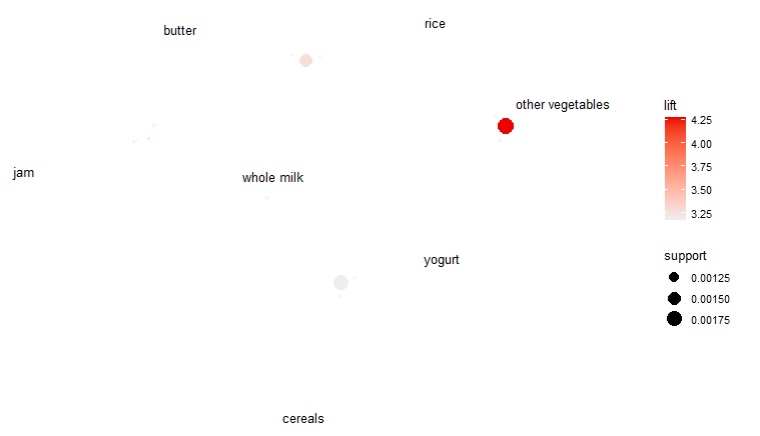 |
연관 네트워크 그래프에서 타원의 크기는 지지도(조합), 색상은 향상도(관련성), 화살표는 상품(item)간의 관계를 나타낸다.
'통계기반 데이터분석' 카테고리의 다른 글
| [ R ] xgboost (0) | 2022.12.05 |
|---|---|
| [ R ] 연관분석 #1 (0) | 2022.12.04 |
| [ R ] 군집분석 #2 (0) | 2022.12.03 |
| [ R ] 군집분석 #1 (0) | 2022.12.03 |
| [ R ] 오분류표 (1) | 2022.12.03 |


