
59doit
[ R ]다양한 시각화 # 6 ggplot 본문
(2) ggplot() 함수
ggplot()함수는 데이터 속성에 미적요소를 매핑한 후 스케일링과정을 거쳐서 생성된 객체를 + 연산자를 사용하여 미적 요소 맵핑을 새로운 레이어에 상속받아 재사용할 수 있도록 지원하는 ggplot2 패키지의 함수
# 미적 요소 맵핑
aes()함수를 이용하여 미적요소만 별도 지정 가능
# 1 aes()함수 속성을 추가하여 미적 요소 맵핑하기
#1-1 데이터 셋에 미적 요소 맵핑 (diamonds 데이터 이용)
| p <- ggplot(diamonds,aes(carat,price, color=cut)) p+geom_point() 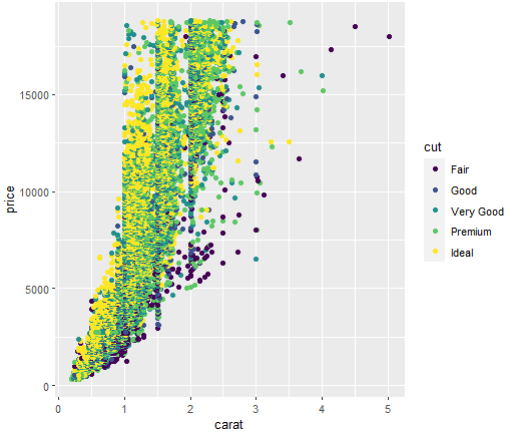 |
#1-2 데이터 셋에 미적 요소 맵핑 (mtcars 데이터 이용)
| p <- ggplot(mtcars, aes(mpg, wt, color = factor(cyl))) p+geom_point()  |
# 기하학적 객체 적용 (mtcars 데이터)
geom()함수는 ggplot()함수에서 정의된 미적요소 맵핑 객체를 상속받아서 서로 다른 레이어에서 별도로 재사용 할 수 있다.
# 2 geom_line()과 geom_point()함수를 적용하여 레이어 추가
#2-1 geom_line()레이어 추가
| p <- ggplot(mtcars,aes(mpg, wt, color=factor(cyl))) p+geom_line()  |
#2-2 geom_point레이어 추가
| p <- ggplot(mtcars,aes(mpg, wt, color=factor(cyl))) p+geom_point()  |
# 미적 요소 맵핑과 기하학적 객체 적용 ( diamonds 데이터 이용 )
stat_bin()함수는 aes()함수와 geom()함수의 기능을 동시에 제공
# 1 stat_bin()함수를 사용하여 막대 그래프 그리기
#1-1 기본 미적 요소 맵핑 객체를 생성한 뒤에 stat_bin()함수 사용
| p <- ggplot(diamonds, aes(price)) p + stat_bin(aes(fill = cut), geom = "bar")  |
#1-2 price빈도를 밀도(전체의 합=1)로 스케일링하여 stat_bin()함수 사용
p + stat_bin(aes(fill = ..density..), geom = "bar") |
cf ) ggplot() 함수에 의해서 그래프가 그려지는 절차
1) 미적요소 맵핑(aes): x 축, y 축, color속성
2) 통계적인 변환(stat): 통계계산 작업
3) 기하학적 객체 적용(geom): 차트 유형
4) 위치조정(position, adjustment), 채우기(fill), 스택(stack), 닷지(dodge) 유형
# 2 stat_bin()함수 적용 영역과 산점도 그래프 그리기
#2-1
| p <- ggplot(diamonds, aes(price)) p + stat_bin(aes(fill = cut), geom = "area")  |
#2-2 stat_bin()함수로 산점도 그래프 그리기
| p + stat_bin(aes(color = cut, size = ..density..), geom = "point")  |
# 산점도와 회귀선 적용 ( galton 데이터 이용 )
회귀선을 시각화하기 위해
geom_count()함수사용 : 숫자의 크기에 따라서 산점도를 시각화
geom_smooth()함수 : 속성으로 method=”lm”을 지정하면 회귀선과 보조선으로 시각화 사용.
| library(UsingR) data("galton") p <- ggplot(data = galton, aes(x = parent, y = child)) p + geom_count() + geom_smooth(method ="lm") 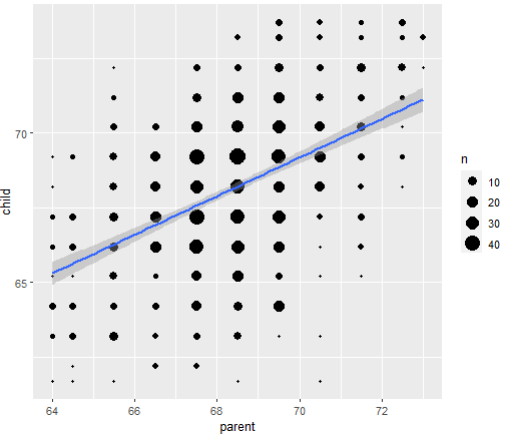 |
# 테마(Theme) 적용
테마: 그래프의 외형 지정
#1 테마를 적용하여 그래프 외형 속성 설정
#1-1 제목을 설정한 산점도 그래프
| p <- ggplot(diamonds, aes(carat, price, color = cut)) p <- p + geom_point() + ggtitle("다이아몬드 무게와 가격의 상관관계") print(p)  |
#1-2 theme()함수를 이용하여 그래프의 외형 속성 적용
| p + theme( title = element_text(color = "blue3", size = 25), axis.title = element_text(size = 10, face ="bold"), axis.title.x = element_text(color = "green3"), axis.title.y = element_text(color = "green3"), axis.text = element_text(size = 10), axis.text.y = element_text(color = "purple"), axis.text.x = element_text(color = "red"), legend.title = element_text(size = 14, face = "bold", color = "darkred"), legend.position = "bottom", legend.direction = "horizontal" )  |
2) ggsave() 함수
그래프를 pdf 또는 이미지 형식( jpg, png 등)의 파일로 저장
이미지의 해상도, 폭, 너비 지정 가능
# 그래프를 이미지 파일로 저장하기
#1 저장할 plot
| p <- ggplot(diamonds, aes(carat, price, color = cut)) p + geom_point()  |
#2 가장 최근에 그려진 그래프 저장
| ggsave(file = "C:/Rwork/output/diamond_price.pdf") ggsave(file = "C:/Rwork/output.diamond_price.jpg", dp = 72) |
#3 변수에 저장된 그래프를 이미지 파일로 저장하기
| p <- ggplot(diamonds, aes(clarity)) p <- p + geom_bar(aes(fill = cut), position = "fill") ggsave(file = "C:/Rwork/output/bar.png", plot = p, width = 10, height = 5) |
'Programming > R' 카테고리의 다른 글
| [ R ]다양한 시각화 # 7 ggsave() & 지도 공간 기법 (0) | 2022.12.24 |
|---|---|
| [ R ] 다양한 시각화 #5 기하학적 기법 시각화 (0) | 2022.12.24 |
| [ R ]다양한 시각화 # 4 조건 그래프 (0) | 2022.12.23 |
| [ R ]다양한 시각화 # 3 데이터범주화 (0) | 2022.12.23 |
| [ R ] 다양한 시각화 #2 점 ㆍ산점도 그래프 (0) | 2022.12.23 |


